In the prior article, we derived the formula for the Living Correlation between 2 data streams. Computing this formula might seem daunting. To perform the necessary calculations, it is necessary to know the current Z scores of 2 data streams plus the most recent correlation.

To dispel the notion that this computation is complicated and beyond the abilities of sophisticated life forms and the mathematically challenged, much less simpler life forms, we are going to take two tacks. First, we are going to examine the computation from the perspective of neural networks. Second, we will discuss how each of us might employ this formula on a daily level to make rough correlations concerning our lives.

Computing the Living Correlation via existing Neural Networks

For the purposes of this discussion, we are going to make two major assumptions. 1) Living systems employ the Living Algorithm’s algorithm to analyze data streams. 2) Living systems have the ability to choose between alternative courses of behavior. We have good reasons for making these assumptions.

In terms of the 1st assumption: 1) the Living Algorithm is the only candidate that fulfills the requirements for the position as Life’s mathematical system. [See Living Algorithm.] 2) There are myriad patterns of correspondence between the Living Algorithm’s mathematical system and the common behavior of living systems. Sleep related behavior and Posner’s Attention Model are just two of many instances.

In terms of the 2nd assumption: There are many types of common human behavior, such as advertising, political campaigns, self-help books, and religion, that are based in the notion that humans have the ability to choose between alternate courses of action. Automatic explanations for these types of behavior from a material, biological, neurological or random perspective are inadequate, offering little, if any, insight into the underlying mechanisms behind these common human patterns. In contrast to the Living Algorithm perspective provides deep insights into these behavior patterns. For these reasons, we feel justified in basing the following discussion upon these two primary assumptions.

We have discussed elsewhere the pragmatic nature of the Living Algorithm (the Living Algorithm) for living systems. The measures generated by the Living Algorithm act as both simple descriptive predictors and as information filters. According to this system, the Living Algorithm is the method by which living systems digest and filter the multitude of data streams that they are constantly bombarded with. The Living Algorithm digests sensory and other types of data streams. The digestion process transforms raw or digested data streams into derivative data streams.

These derivative data streams provide many evolutionary advantages to living systems. For the purposes of this discussion, we will provide just two. First, employing the Living Algorithm saves an enormous amount of precious memory space. Instead of remembering all environmental input, the organism is only required to retain the most recent information from the derivative data streams. Once it has been digested, raw data is immediately discarded. The raw data serves no further purpose, as the Living Algorithm automatically incorporates the information it contains into the derivative data streams.

This brings us to the second advantage. The Living Algorithm digests data streams transforming them into derivative data streams that describe the location, range and tendency of the current moment. This descriptive information is employed to make predictions regarding the next data point in the stream. While imprecise, these measures, like the weather forecast, narrow the range of likely possibilities tremendously. This limitation of the range of possibility enables the organism to save energy and enhances the possibility of success.

There are 3 primary derivative data streams: 1) the Living Average (position), 2) the Deviation (range), and the Directional (tendency). According to the theory, living systems automatically digest raw data streams to obtain these 3 derivative data streams. Just as with the raw data, all the past information from the derivative data streams is immediately discarded as it is immediately incorporated into the most recent figures. In other words, the digestion process generates 3 basic figures. Living systems are only required to retain these figures, as they are the most relevant in terms of describing the trajectories of the present moment and thereby predicting the next moment.

To compute the Living Z-score of the current moment, the organism only requires the Raw Data and the memory of 2 of these composite numbers, i.e. the Living Average and the Deviation. Recall the simple formula: take the difference between the New Data point and the past Living Average and then divide by the past Deviation. This yields the current Z-score.

Computing the Z-score provides information that has inherent utility for the organism. Employing the Living Algorithm on the Z-score generates another data stream. If the Z-score data stream rises above 1, it is an indication that there is a change in the environment, as the most probable range is less than positive or negative 1. The organism must attend to environmental changes in order to facilitate survival. The change might indicate predator or prey. We can imagine that with the increase in brainpower that living systems could have easily added this information to their bag of useful data stream measures.

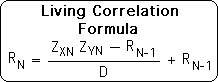
Once the organism retains the Z-score, it is a straightforward step to then calculate the Living Correlation between 2 data streams. Compute the Product of the most recent Z-scores from the relevant data streams. Take the Difference between this product and the past Correlation, divide by the Decay Factor, and then add this value to the past Correlation. This computational process would be easy for the organism as it is just another form of the Living Algorithm. The only difference is that the product of the Z-scores acts as the Current or Raw Data.

Although a simple extension, we imagine that it would require another increase in neural capacity to attend to this additional data stream.

We suggest that Attention increases with neural capacity. The greater the neural capacity; the greater the ability to attend to an increasing number and types of data streams. The simplest organisms can only attend to a few types data streams. This simplest form of Attention employs the Living Algorithm to digest data streams into the 3 basic derivative data streams. The reactions and modifications are relatively automatic.

Random genetic mutations eventually led to an increase in brain size. While some of this increase had to do with biological functions, some of the increase had to do with computational ability. With the enhanced storage capacity, more data streams could be digested. The visual cortex evolved to deal with sensory input from the eyes. While some of the increase had to do with the number of data streams, some of the increase concerned the type of data stream.

From the computation of the Living Average and Deviation, it just took a single mutative genetic leap to begin computing the Z-score data stream. Or it might have been an emergent feature of increased brainpower. With another jump in brainpower, two data streams could have been attended to simultaneously. With this increase in Attention, two Z-score data streams could have been easily combined to generate the Correlation data stream. Again this jump could have been due to genetic mutation, emergence or a combination of both. Whichever way it occurred, this increased knowledge would have certainly provided an evolutionary advantage.

Approximating Living Correlations in Day-to-Day Life

Now let us look at how we might employ the seemingly complicated equation for correlations in our ordinary day-to-day lives.

The Standard Deviations, Mean Averages and Z-scores that it takes to compute Correlations seem exceedingly complicated. As an indication of the difficulty of computation, these measures are generally only introduced in college level probability and statistic classes. These measures are only applicable to data sets. Due to the number of elements in even a small data set, numerous calculations, including a square root, are required to determine the correlation.

Let us consider a simple example. We would like to know the correlation between sets X and Y. Assume that our data sets, both have 10 members. For the Mean Average, we must sum up the elements and then divide by N, the number of elements, in this case 10 (2 computations). To obtain the Standard Deviation of Set X, we subtract each element from the average, square them, add them up, divide by N and then take the square root (23 computations). To determine the Z-scores, we must divide each of the data/average differences by the Standard Deviation (10 more computations). In brief, it takes 35 computations to determine the Z-scores for just one set. To determine the Z-scores for Set Y, we must perform the same 35 computations.

To determine the correlation between the sets, the 10 Z-scores from each set must then be multiplied together, summed, and then divided by N (another 12 computations). In other words it takes 82 computations to determine the correlation between two 10-element data sets. Further, each of the 20 data points and their position in the set must be ‘remembered’ or recorded precisely in order to arrive at the proper figure. It is no wonder that college and computers are required to compute correlations between data sets. Due to the number of computations combined with precise memory requirements, it is hard to imagine how living systems could possibly compute correlations rapidly enough to have any immediate relevance for survival.

Let us consider a simple example. First, living systems are comparing data streams, not data sets. To determine the correlation between 2 data streams, the organism only has to compute and ‘remember’ 4 figures from each data stream (8 in all). The Living Algorithm computes three of these measures – the Living Average, the Deviation, and the Correlation. In other words, a single, regularly used process is employed to generate the relevant figures. Two of these measures are required to compute the 4th measure, the Z-score. The Living Algorithm then operates on the product of the current Z-scores to determine the current Correlation. Due to the repetition of one process, the computational requirements are minimal.

The memory requirements are equally small. Although data streams go on virtually forever, the number of elements in the stream is not part of the equation. It is not a difficult task to ‘remember’ the relevant measures as each of these figures is emotionally charged due to the fact that they provide relevant information regarding the data stream.

Let’s see a pragmatic application of these processes. Each of us employs the Living Algorithm to determine the probable time of arrival and the probable range of variation of fellow employees, students, friends, and partners. For instance, if we regularly have lunch with a friend, most of us have a distinct sense whether our meal partner tends to be late, on time, or early. Further, we could also provide a plus or minus to the expected arrival time. If queried, we might say: “He always shows up about 10 minutes late, plus or minus 5 minutes.” These figures are rough, yet pragmatic, estimates of the Living Average and the Deviation.

It is an easy step for most of us to say, “He was really late today because he showed up 20 minutes after the appointed lunch time.” or “Wow! He showed up on time. That was certainly unexpected.” These statements indicate that we also have a distinct sense of Z-scores.

We instantly know that our partner’s current Z-score is over 1, as he has exceeded the normal limits of his arrival time. Further, no one has to inform us that this new arrival time is unusual. If he continues to show up exceptionally late or early, we will probably begin adjusting his expected arrival time and the range.

Or we might even ask if something has changed in his life to alter his behavior outside the ordinary. The latter query indicates that we are well aware of correlations with other data streams. Most of us understand computationally and/or experientially that well-established behavior patterns don’t change unless there is a change in external circumstances or internal attitude.

Suppose that our spouse always shows up at 6PM plus or minus 10 minutes after work. Then suppose a new data stream enters the consciousness – alcohol on the breath. Suppose that every time, our spouse shows up later than usual that he has alcohol on his breath. In contrast, when he shows up on time, there is no odor. With an increasing number of instances, we begin to sense a correlation between drinking and a late arrival time. We have almost instinctively been computing pragmatic correlations between the arrival time data stream and the drinking data stream. We easily remembered the relevant measures because they were important and equally easily made the relevant calculations, as they are hard-wired into our cognitive system.

This example is fairly blunt. Due to the sophistication of our neural networks we have data streams for facial gestures, voice intonation and body posture. Due to the pragmatic nature of the Living Algorithm, we immediately compute the probable location and range of these data streams. With this information, we can then compute Z-scores that indicate unusual data points. By comparing the Z-scores of relevant data stream, we can then easily compute correlations. For instance, a tense body posture is correlated with angry words, while a relaxed body posture might be correlated with friendly words. All of us regularly compute Living Correlations to make better predictions regarding the circumstances of our lives. Due to these predictions, we are able to make more effective responses to our friends and family.

Many animals have the ability to compute correlations. Humans have other computational abilities that are unique to our species.